Pallas Quickstart

Pallas is an extension to JAX that enables writing custom kernels for GPU and TPU. Pallas allows you to use the same JAX functions and APIs but operates at a lower level of abstraction.

Specifically, Pallas requires users to think about memory access and how to divide up computations across multiple compute units in a hardware accelerator. On GPUs, Pallas lowers to Triton and on TPUs, Pallas lowers to Mosaic.

Let’s dive into some examples.

Note: Pallas is still an experimental API and you may be broken by changes!

Hello world in Pallas

from functools import partial

import jax
from jax.experimental import pallas as pl
import jax.numpy as jnp
import numpy as np

We’ll first write the “hello world” in Pallas, a kernel that adds two vectors.

def add_vectors_kernel(x_ref, y_ref, o_ref):
  x, y = x_ref[...], y_ref[...]
  o_ref[...] = x + y

Ref types

Let’s dissect this function a bit. Unlike most JAX functions you’ve probably written, it does not take in jax.Arrays as inputs and doesn’t return any values. Instead it takes in Ref objects as inputs. Note that we also don’t have any outputs but we are given an o_ref, which corresponds to the desired output.

Reading from Refs

In the body, we are first reading from x_ref and y_ref, indicated by the [...] (the ellipsis means we are reading the whole Ref; alternatively we also could have used x_ref[:]). Reading from a Ref like this returns a jax.Array.

Writing to Refs

We then write x + y to o_ref. Mutation has not historically been supported in JAX – jax.Arrays are immutable! Refs are new (experimental) types that allow mutation under certain circumstances. We can interpret writing to a Ref as mutating its underlying buffer.

So we’ve written what we call a “kernel”, which we define as a program that will run as an atomic unit of execution on an accelerator, without any interaction with the host. How do we invoke it from a JAX computation? We use the pallas_call higher-order function.

@jax.jit
def add_vectors(x: jax.Array, y: jax.Array) -> jax.Array:
  return pl.pallas_call(add_vectors_kernel,
                        out_shape=jax.ShapeDtypeStruct(x.shape, x.dtype)
                        )(x, y)
add_vectors(jnp.arange(8), jnp.arange(8))

Array([ 0,  2,  4,  6,  8, 10, 12, 14], dtype=int32)

pallas_call lifts the Pallas kernel function into an operation that can be called as part of a larger JAX program. But, to do so, it needs a few more details. Here we specify out_shape, an object that has a .shape and .dtype (or a list thereof). out_shape determines the shape/dtype of o_ref in our add_vector_kernel.

pallas_call returns a function that takes in and returns jax.Arrays.

What’s actually happening here?

Thus far we’ve described how to think about Pallas kernels but what we’ve actually accomplished is we’re writing a function that’s executed very close to the compute units.

On GPU, x_ref corresponds to a value in high-bandwidth memory (HBM) and when we do x_ref[...] we are copying the value from HBM into static RAM (SRAM) (this is a costly operation generally speaking!). We then use GPU vector compute to execute the addition, then copy the resulting value in SRAM back to HBM.

On TPU, we do something slightly different. Before the kernel is ever executed, we fetch the value from HBM into SRAM. x_ref therefore corresponds to a value in SRAM and when we do x_ref[...] we are copying the value from SRAM into a register. We then use TPU vector compute to execute the addition, then copy the resulting value back into SRAM. After the kernel is executed, the SRAM value is copied back into HBM.

We are in the process of writing backend-specific Pallas guides. Coming soon!

Pallas programming model

In our “hello world” example, we wrote a very simple kernel. It takes advantage of the fact that our 8-sized arrays can comfortably fit inside the SRAM of hardware accelerators. In most real-world applications, this will not be the case!

Part of writing Pallas kernels is thinking about how to take big arrays that live in high-bandwidth memory (HBM, also known as DRAM) and expressing computations that operate on “blocks” of those arrays that can fit in SRAM.

Grids

To automatically “carve” up the inputs and outputs, you provide a grid and BlockSpecs to pallas_call.

A grid is a tuple of integers (e.g. (), (2, 3, 4), or (8,)) that specifies an iteration space. For example, a grid (4, 5) would have 20 elements: (0, 0), (0, 1), ..., (0, 4), (1, 0), ..., (3, 4). We run the kernel function once for each element, a style of single-program multiple-data (SPMD) programming.

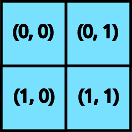
A 2D grid

When we provide a grid to pallas_call, the kernel is executed as many times as prod(grid). Each of these invocations is referred to as a “program”, To access which program (i.e. which element of the grid) the kernel is currently executing, we use program_id(axis=...). For example, for invocation (1, 2), program_id(axis=0) returns 1 and program_id(axis=1) returns 2.

Here’s an example kernel that uses a grid and program_id.

def iota_kernel(o_ref):
  i = pl.program_id(0)
  o_ref[i] = i

We now execute it using pallas_call with an additional grid argument.

def iota(len: int):
  return pl.pallas_call(iota_kernel,
                        out_shape=jax.ShapeDtypeStruct((len,), jnp.int32),
                        grid=(len,))()
iota(8)

Array([0, 1, 2, 3, 4, 5, 6, 7], dtype=int32)

On GPUs, each program is executed in parallel on separate threads. Thus, we need to think about race conditions on writes to HBM. A reasonable approach is to write our kernels in such a way that different programs write to disjoint places in HBM to avoid these parallel writes. On the other hand, parallelizing the computation is how we can execute operations like matrix multiplications really quickly.

On TPUs, programs are executed in a combination of parallel and sequential (depending on the architecture) so there are slightly different considerations.

Block specs

With grid and program_id in mind, Pallas provides an abstraction that takes care of some common indexing patterns seen in a lot of kernels. To build intuition, let’s try to implement a matrix multiplication.

A simple strategy for implementing a matrix multiplication in Pallas is to implement it recursively. We know our underlying hardware has support for small matrix multiplications (using GPU and TPU tensorcores), so we just express a big matrix multiplication in terms of smaller ones.

Suppose we have input matrices \(X\) and \(Y\) and are computing \(Z = XY\). We first express \(X\) and \(Y\) as block matrices. \(X\) will have “row” blocks and \(Y\) will have “column” blocks.

\[\begin{split} \begin{align*} X = \begin{bmatrix} X_0 \\ X_1 \end{bmatrix} \end{align*} \end{split}\]

\[ \begin{align*} Y = \begin{bmatrix} Y_0 & Y_1 \end{bmatrix} \end{align*} \]

\[\begin{split} \begin{align*} Z &= \begin{bmatrix} X_0 \\ X_1 \end{bmatrix} \begin{matrix} \begin{bmatrix} Y_0 & Y_1 \end{bmatrix} \\ ~ \end{matrix} \\ &= \begin{bmatrix} X_0 Y_0 & X_0 Y_1 \\ X_1 Y_0 & X_1 Y_1 \end{bmatrix} \end{align*} \end{split}\]

Our strategy is that because \(Z\) is also a block matrix, we can assign each of the programs in our Pallas kernel one of the output blocks. Computing each output block corresponds to doing a smaller matrix multiply between a “row” block of \(X\) and a “column” block of \(Y\).

To express this pattern, we use BlockSpecs. A BlockSpec specifies a block shape for each input and output, and an “index map” function, that maps a set of program indices to a block index.

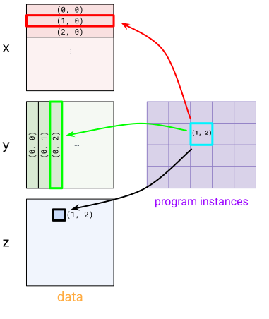
A visualization of a BlockSpec

For a concrete example, let’s say we’d like to multiply two (1024, 1024) matrices x and y together to produce z, and would like to parallelize the computation 4 ways. We split up z into 4 (512, 512) blocks where each block is computed with a (512, 1024) x (1024, 512) matrix multiplication. To express this, we’d first use a (2, 2) grid (one block for each program).

For x, we use BlockSpec(lambda i, j: (i, 0), (512, 1024)) – this carves x up into “row” blocks. To see this see how both program instances (1, 0) and (1, 1) pick the (1, 0) block in x. For y, we use a transposed version BlockSpec(lambda i, j: (0, j), (1024, 512)). Finally, for z we use BlockSpec(lambda i, j: (i, j), (512, 512)).

These BlockSpecs are passed into pallas_call via in_specs and out_specs.

Underneath the hood, pallas_call will automatically carve up your inputs and outputs into Refs for each block that will be passed into the kernel.

def matmul_kernel(x_ref, y_ref, z_ref):
  z_ref[...] = x_ref[...] @ y_ref[...]

def matmul(x: jax.Array, y: jax.Array):
  return pl.pallas_call(
    matmul_kernel,
    out_shape=jax.ShapeDtypeStruct((x.shape[0], y.shape[1]), x.dtype),
    grid=(2, 2),
    in_specs=[
      pl.BlockSpec(lambda i, j: (i, 0), (x.shape[0] // 2, x.shape[1])),
      pl.BlockSpec(lambda i, j: (0, j), (y.shape[0], y.shape[1] // 2))
    ],
    out_specs=pl.BlockSpec(
      lambda i, j: (i, j), (x.shape[0] // 2, y.shape[1] // 2)
    )
  )(x, y)
k1, k2 = jax.random.split(jax.random.key(0))
x = jax.random.normal(k1, (1024, 1024))
y = jax.random.normal(k2, (1024, 1024))
z = matmul(x, y)
np.testing.assert_allclose(z, x @ y)

Note that this is a very naive implementation of a matrix multiplication but consider it a starting point for various types of optimizations. Let’s add an additional feature to our matrix multiply: fused activation. It’s actually really easy! Just pass a higher-order activation function into the kernel.

def matmul_kernel(x_ref, y_ref, z_ref, *, activation):
  z_ref[...] = activation(x_ref[...] @ y_ref[...])

def matmul(x: jax.Array, y: jax.Array, *, activation):
  return pl.pallas_call(
    partial(matmul_kernel, activation=activation),
    out_shape=jax.ShapeDtypeStruct((x.shape[0], y.shape[1]), x.dtype),
    grid=(2, 2),
    in_specs=[
      pl.BlockSpec(lambda i, j: (i, 0), (x.shape[0] // 2, x.shape[1])),
      pl.BlockSpec(lambda i, j: (0, j), (y.shape[0], y.shape[1] // 2))
    ],
    out_specs=pl.BlockSpec(
      lambda i, j: (i, j), (x.shape[0] // 2, y.shape[1] // 2)
    ),
  )(x, y)
k1, k2 = jax.random.split(jax.random.key(0))
x = jax.random.normal(k1, (1024, 1024))
y = jax.random.normal(k2, (1024, 1024))
z = matmul(x, y, activation=jax.nn.relu)
np.testing.assert_allclose(z, jax.nn.relu(x @ y))

To conclude, let’s highlight a cool feature of Pallas: it composes with jax.vmap! To turn this matrix multiplication into a batched version, we just need to vmap it.

k1, k2 = jax.random.split(jax.random.key(0))
x = jax.random.normal(k1, (4, 1024, 1024))
y = jax.random.normal(k2, (4, 1024, 1024))
z = jax.vmap(partial(matmul, activation=jax.nn.relu))(x, y)
np.testing.assert_allclose(z, jax.nn.relu(jax.vmap(jnp.matmul)(x, y)))