shmap (shard_map) for simple per-device code#
sholto@, sharadmv@, jekbradbury@, zhangqiaorjc@, mattjj@
January 2023
Motivation#
JAX supports two schools of thought for multi-device programming:
Compiler, take the wheel! Let the compiler automatically partition bulk array functions over devices.
Just let me write what I mean, damnit! Give me per-device code and explicit communication collectives.
We need great APIs for both, and rather than being mutually exclusive alternatives, they need to compose with each other.
With pjit (now just jit) we have a next-gen
API
for the first school. But we haven’t quite leveled-up the second school. pmap
follows the second school, but over time we found it has fatal
flaws. xmap solved those flaws,
but it doesn’t quite give us per-device shapes, and it includes several other
big ideas too. Meanwhile, new demands for per-device explicit-collectives
programming have emerged, like in Efficiently Scaling Transformer
Inference.
We can level-up the second school with shmap. shmap is:
a simple multi-device parallelism API which lets us write per-device code with explicit collectives, where logical shapes match per-device physical buffer shapes and collectives correspond exactly to cross-device communication;
a specialization of
xmapwith scaled-back features and a few tweaks;a fairly direct surfacing of the XLA SPMD Partitioner’s ‘manual’ mode;
a fun-to-say Seussian name which could stand for
shard_map,shpecialized_xmap,sholto_map, orsharad_map.
For pjit users, shmap is a complementary tool. It can be used inside a
pjit computation to drop temporarily into a “manual collectives” mode, like an
escape hatch from the compiler’s automatic partitioning. That way, users get the
convenience and familiar just-NumPy programming model of pjit for most of their
code, along with the ability to hand-optimize collective communication with
shmap wherever it’s needed. It’s the best of both worlds!
For pmap users, shmap is a strict upgrade. It’s more expressive,
performant, and composable with other JAX APIs, without making basic batch data
parallelism any harder.
For more on practical use, you can jump to When should you use shmap and when
should you use pjit?.
If you’re wondering why we need a new thing at all, or what
the problems with pmap are, jump to Why don’t pmap or xmap already solve
this?.
Or keep reading the next section to see some shmap examples and the API spec.
So, let’s see shmap!#
TL;DR example (with a more detailed explanation to follow)#
Sho shick:
from functools import partial

import numpy as np

import jax
import jax.numpy as jnp
from jax.sharding import Mesh, PartitionSpec as P
from jax.experimental import mesh_utils
from jax.experimental.shard_map import shard_map

devices = mesh_utils.create_device_mesh((4, 2))
mesh = Mesh(devices, axis_names=('i', 'j'))

a = jnp.arange( 8 * 16.).reshape(8, 16)
b = jnp.arange(16 * 32.).reshape(16, 32)

@partial(shard_map, mesh=mesh, in_specs=(P('i', 'j'), P('j', None)),
         out_specs=P('i', None))
def matmul_basic(a_block, b_block):
  # a_block: f32[2, 8]
  # b_block: f32[8, 32]
  z_partialsum = jnp.dot(a_block, b_block)
  z_block = jax.lax.psum(z_partialsum, 'j')
  return z_block

c = matmul_basic(a, b)  # c: f32[8, 32]
Notice:
no nesting needed (or
axis_index_groups) for multiple axes of parallelism, unlikepmap;no reshapes in the caller, unlike
pmapand hard-xmap, and logical shapes correspond to per-device physical shapes, unlike (non-hard)xmap;precise device placement control by using
mesh, unlikepmap;there’s only one set of axis names for logical and physical, unlike
xmap;the result is a
jax.Arraywhich could be efficiently passed to apjit, unlikepmap;this same code works efficiently inside a
pjit/jit, unlikepmap;this code works eagerly, so we can
pdbin the middle and print values, unlikexmap’s current implementation (though by designxmapwithout the sequential schedule can in principle work eagerly too).
Here’s another matmul variant with a fully sharded result:
@partial(shard_map, mesh=mesh, in_specs=(P('i', 'j'), P('j', None)),
         out_specs=P('i', 'j'))
def matmul_reduce_scatter(a_block, b_block):
  # c_partialsum: f32[8/X, 32]
  c_partialsum = jnp.matmul(a_block, b_block)
  # c_block: f32[8/X, 32/Y]
  c_block = jax.lax.psum_scatter(c_partialsum, 'j', scatter_dimension=1, tiled=True)
  return c_block

c = matmul_reduce_scatter(a, b)
Slow down, start with the basics!#
Rank-reducing vs rank-preserving maps over array axes#
We can think of pmap (and vmap and xmap) as unstacking each array input
along an axis (e.g. unpacking a 2D matrix into its 1D rows), applying its body
function to each piece, and stacking the results back together, at least when
collectives aren’t involved:
pmap(f, in_axes=[0], out_axes=0)(xs) == jnp.stack([f(x) for x in xs])
For example, if xs had shape f32[8,5] then each x has shape f32[5], and
if each f(x) has shape f32[3,7] then the final stacked result pmap(f)(xs)
has shape f32[8,3,7]. That is, each application of the body function f takes
as argument inputs with one fewer axis than the corresponding argument to
pmap(f). We can say these are rank-reducing maps with unstacking/stacking of
inputs/outputs.
The number of logical applications of f is determined by the size of the input
axis being mapped over: for example, if we map over an input axis of size 8,
semantically we get 8 logical applications of the function, which for pmap
always correspond to 8 devices physically computing them.
In contrast, shmap does not have this rank-reducing behavior. Instead, we can
think of it as slicing (or “unconcatenating”) along input axes into blocks,
applying the body function, and concatenating the results back together (again
when collectives aren’t involved):
devices = np.array(jax.devices()[:4])
m = Mesh(devices, ('i',))  # mesh.shape['i'] = 4

shard_map(f, m, in_specs=P('i'), out_specs=P('i'))(y)
==
jnp.concatenate([f(y_blk) for y_blk in jnp.split(y, 4)])
Recall that jnp.split slices its input into equally-sized blocks with the same
rank, so that if in the above example y has shape f32[8,5] then each y_blk
has shape f32[2,5], and if each f(y_blk) has shape f32[3,7] then the final
concatenated result shard_map(f, ...)(y) has shape f32[12,7]. So shmap
(shard_map) maps over shards, or blocks, of its inputs. We can say it’s a
rank-preserving map with unconcatenating/concatenating of its inputs/outputs.
The number of logical applications of f is determined by the mesh size, not by
any input axis size: for example, if we have a mesh of total size 4 (i.e. over 4
devices) then semantically we get 4 logical applications of the function,
corresponding to the 4 devices physically computing them.
Controlling how each input is split (unconcatenated) and tiled with in_specs#
Each of the in_specs identifies some of the corresponding input array’s axes
with mesh axes by name using PartitionSpecs, representing how to split (or
unconcatenate) that input into the blocks to which the body function is applied.
That identification determines the shard sizes; when an input axis is identified
with a mesh axis, the input is split (unconcatenated) along that logical axis
into a number of pieces equal to the corresponding mesh axis size. (It’s an
error if the corresponding mesh axis size does not evenly divide the input array
axis size.) If an input’s pspec does not mention a mesh axis name, then there’s
no splitting over that mesh axis. For example:
devices = np.array(jax.devices())
m = Mesh(devices.reshape(4, 2), ('i', 'j'))

@partial(shard_map, mesh=m, in_specs=P('i', None), out_specs=P('i', 'j'))
def f1(x_block):
  print(x_block.shape)
  return x_block

x1 = np.arange(12 * 12).reshape(12, 12)
y = f1(x1)  # prints (3,12)
Here, because the input pspec did not mention the mesh axis name 'j', no input
array axis is split over that mesh axis; similarly, because the second axis of
the input array is not identified with (and hence split over) any mesh axis,
application of f1 gets a full view of the input along that axis.
When a mesh axis is not mentioned in an input pspec, we can always rewrite to a
less efficient program where all mesh axes are mentioned but the caller performs
a jnp.tile, for example:
@partial(shard_map, mesh=m, in_specs=P('i', 'j'), out_specs=P('i', 'j'))
def f2(x_block):
  print(x_block.shape)
  return x_block

x = np.arange(12 * 12).reshape(12, 12)
x_ = jnp.tile(x, (1, mesh.axis_size['j']))  # x_ has shape (12, 24)
y = f2(x_)  # prints (3,12), and f1(x) == f2(x_)
In other words, because each input pspec can mention each mesh axis name zero or
one times, rather than having to mention each name exactly once, we can say that
in addition to the jnp.split built into its input, shard_map also has a
jnp.tile built into its input, at least logically (though the tiling may not
need to be carried out physically, depending on the arguments’ physical sharding
layout). The tiling to use is not unique; we could also have tiled along the
first axis, and used the pspec P(('j', 'i'), None).
Physical data movement is possible on inputs, as each device needs to have a copy of the appropriate data.
Controlling how each output assembled by concatenation, block transposition, and untiling using out_specs#
Analogously to the input side, each of the out_specs identifies some of the
corresponding output array’s axes with mesh axes by name, representing how the
output blocks (one for each application of the body function, or equivalently
one for each physical device) should be assembled back together to form the
final output value. For example, in both the f1 and f2 examples above the
out_specs indicate we should form the final output by concatenating together
the block results along both axes, resulting in both cases an array y of shape
(12,24). (It’s an error if an output shape of the body function, i.e. an
output block shape, has a rank too small for the concatenation described by the
corresponding output pspec.)
When a mesh axis name is not mentioned in an output pspec, it represents an un-tiling: when the user writes an output pspec which does not mention one of the mesh axis names, they promise that the output blocks are equal along that mesh axis, and so only one block along that axis is used in the output (rather than concatenating all the blocks together along that mesh axis). For example, using the same mesh as above:
x = jnp.array([[3.]])

z = shard_map(lambda: x, mesh=m, in_specs=(), out_specs=P('i', 'j'))()
print(z)  # prints the same as jnp.tile(x, (4, 2))

z = shard_map(lambda: x, mesh=m, in_specs=(), out_specs=P('i', None))()
print(z)  # prints the same as jnp.tile(x, (4, 1)), or just jnp.tile(x, (4,))

z = shard_map(lambda: x, mesh=m, in_specs=(), out_specs=P(None, None))()
print(z)  # prints the same as jnp.tile(x, (1, 1)), or just x
Notice that the body function closing over an array value is equivalent to
passing it as an augment with a corresponding input pspec of P(None, None). As
another example, following more closely to the other examples above:
@partial(shard_map, mesh=m, in_specs=P('i', 'j'), out_specs=P('i', None))
def f3(x_block):
  return jax.lax.psum(x_block, 'j')

x = np.arange(12 * 12).reshape(12, 12)
y3 = f3(x)
print(y3.shape)  # (12,6)
Notice that the result has a second axis size of 6, half the size of the input’s
second axis. In this case, the un-tile expressed by not mentioning the mesh axis
name 'j' in the output pspec was safe because of the collective psum, which
ensures each output block is equal along the corresponding mesh axis. Here are
two more examples where we vary which mesh axes are mentioned in the output
pspec:
@partial(shard_map, mesh=m, in_specs=P('i', 'j'), out_specs=P(None, 'j'))
def f4(x_block):
  return jax.lax.psum(x_block, 'i')

x = np.arange(12 * 12).reshape(12, 12)
y4 = f4(x)
print(y4.shape)  # (3,12)


@partial(shard_map, mesh=m, in_specs=P('i', 'j'), out_specs=P(None, None))
def f5(x_block):
  return jax.lax.psum(x_block, ('i', 'j'))

y5 = f5(x)
print(y5.shape)  # (3,6)
On the physical side, not mentioning a mesh axis name in an output pspec
assembles an Array from the output device buffers with replicated layout along
that mesh axis.
There is no runtime check that the output blocks are actually equal along a mesh axis to be un-tiled along, or equivalently that the corresponding physical buffers have equal values and thus can be interpreted as a replicated layout for a single logical array. But we can provide a static check mechanism which raises an error on all potentially-incorrect programs.
Because the out_specs can mention mesh axis names zero or one times, and
because they can be mentioned in any order, we can say that in addition to the
jnp.concatenate built into its output, shard_map also has both an untile and
a block transpose built into its output.
Physical data movement is not possible on outputs, no matter the output pspec.
Instead, out_specs just encodes how to assemble the block outputs into
Arrays, or physically how to interpret the buffers across devices as the
physical layout of a single logical Array.
API Specification#
from jax.sharding import Mesh
Specs = PyTree[PartitionSpec]

def shard_map(f: Callable, mesh: Mesh, in_specs: Specs, out_specs: Specs
          ) -> Callable:
  ...
where:
meshencodes devices arranged in an array and with associated axis names, just like it does forxmapand forsharding.NamedSharding;in_specsandout_specsarePartitionSpecs which can affinely mention axis names frommesh(not separate logical names as inxmap) to express slicing/unconcatenation and concatenation of inputs and outputs, respectively (not unstacking and stacking likepmapandxmapdo), with unmentioned names corresponding to replication and untiling (assert-replicated-so-give-me-one-copy), respectively;the shapes of the arguments passed to
fhave the same ranks as the arguments passed toshard_map-of-f(unlikepmapandxmapwhere the ranks are reduced), and the shape of an argument tofis computed from the shapeshapeof the corresponding argument toshard_map-of-fand the correspondingPartitionSpecspec as roughlytuple(sz // (1 if n is None else mesh.shape[n]) for sz, n in zip(shape, spec));the body of
fcan apply collectives using names frommesh.
shmap is eager by default, meaning that we dispatch computations
primitive-by-primitive, so that the user can employ Python control flow on fully
replicated values and interactive pdb debugging to print any values. To stage
out and end-to-end compile a shmapped function, just put a jit around it. A
consequence is that shmap doesn’t have its own dispatch and compilation paths
like xmap and pmap currently do; it’s just the jit path.
When it’s staged out by e.g. an enclosing jit, the lowering of shmap to
StableHLO is trivial: it just involves switching into ‘manual SPMD mode’ on the
inputs, and switching back on the outputs. (We don’t currently plan to support
partially-manual-partially-automatic modes.)
The interaction with effects is the same as with pmap.
The interaction with autodiff is also just like pmap (rather than attempting
the new semantics that xmap did, corresponding to having unmapped
intermediates and hence grad’s reduce_axes as well as making psum
transpose to pbroadcast rather than psum). But it thus inherits an unsolved
problem from pmap: in some cases, instead of transposing psum to psum, and
thus performing a backward pass psum corresponding to the forward pass psum,
it can be beneficial to move the backward pass psum to elsewhere in the
backward pass, exploiting linearity. Many advanced pmap users addressed this
challenge by using custom_vjp to implement psum_idrev and id_psumrev
functions, but since it’s easy to accidentally leave those imbalanced, that
technique is a foot-cannon. We have some ideas on how to provide this
functionality in a safer way.
When should you use shmap and when should you use pjit?#
One philosophy is: it is almost always simpler to write a program in jit==pjit
— but if a given part of the program is less optimized by the compiler than it
could be, drop into shmap!
A realistic transformer example#
In fact, we can implement a simple version of the “collective
matmul” algorithm
recently introduced in XLA to overlap communication and computation using shmap
and 30 lines of Python. The basic idea of the algorithm can be grasped with a
simple example.
Suppose we want to compute C = A @ B where A is sharded by a 1D mesh on the
0-th dimension while B and C are replicated.
M, K, N = 4096, 2048, 1024
A = jnp.arange(np.prod((M, K))).reshape((M, K))
B = jnp.arange(np.prod((K, N))).reshape((K, N))

mesh = Mesh(np.array(jax.devices()), axis_names=('i'))
A_x = jax.device_put(A, NamedSharding(mesh, P('i', None)))

@jax.jit
def f(lhs, rhs):
  return lhs @ rhs

C = f(A_x, B)
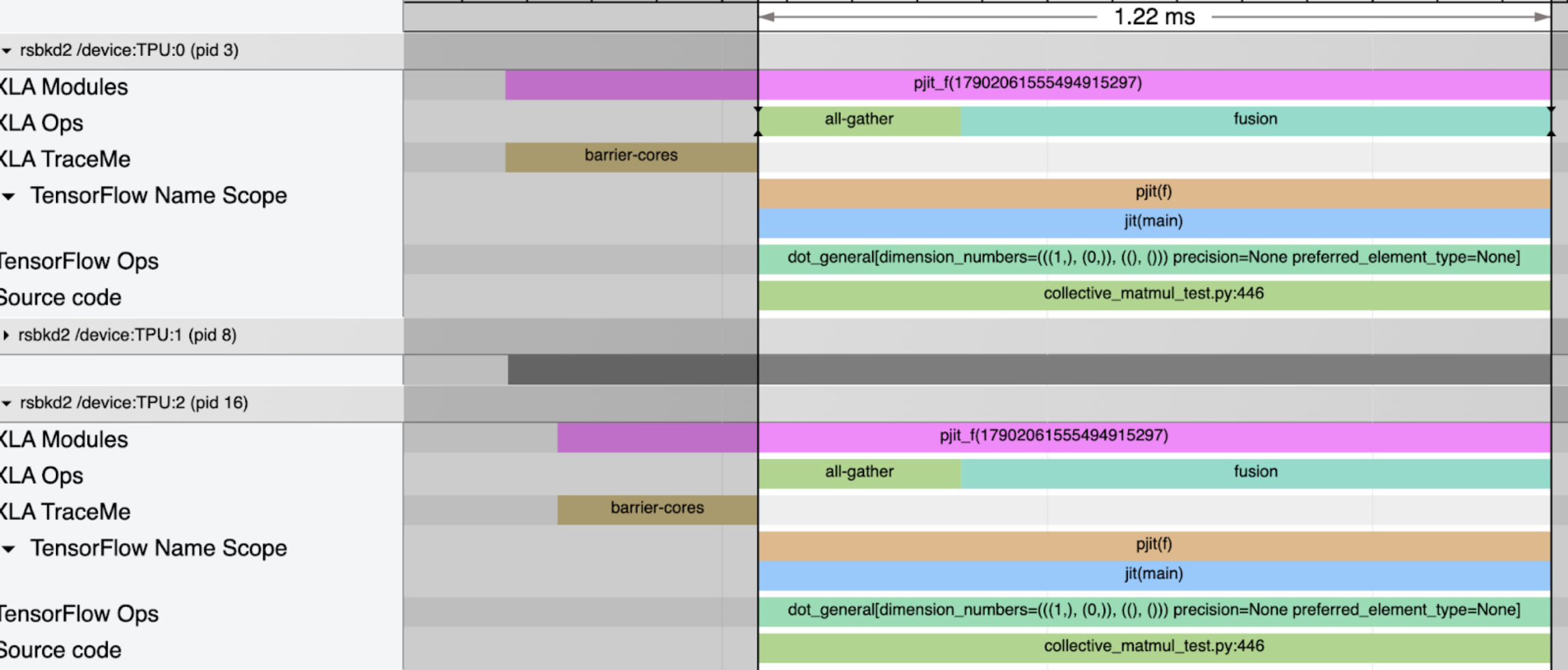
A profile shows the blocking all-gather across 8 devices before the matmul can
start. This is suboptimal because A is sharded on a non-contracting dimension,
and each shard of A can be matmul’ed with B independently and this chunked
computation can be overlapped with fetching of the next shard of A from
another device.
This overlap can be implemented using shmap and explicit collectives.
def collective_matmul_allgather_lhs_non_contracting(lhs, rhs):
  # lhs is the looped operand; rhs is the local operand
  axis_size = jax.lax.psum(1, axis_name='i')
  axis_index = jax.lax.axis_index(axis_name='i')
  chunk_size = lhs.shape[0]

  def f(i, carrys):
    accum, lhs = carrys
    # matmul for a chunk
    update = lhs @ rhs
    # circular shift to the left
    lhs = jax.lax.ppermute(
        lhs,
        axis_name='i',
        perm=[(j, (j - 1) % axis_size) for j in range(axis_size)]
    )
    # device 0 computes chunks 0, 1, ...
    # device 1 computes chunks 1, 2, ...
    update_index = (((axis_index + i) % axis_size) * chunk_size, 0)
    accum = jax.lax.dynamic_update_slice(accum, update, update_index)
    return accum, lhs

  accum = jnp.zeros((lhs.shape[0] * axis_size, rhs.shape[1]), dtype=lhs.dtype)
  # fori_loop cause a crash: hlo_sharding.cc:817 Check failed: !IsManual()
  # accum, lhs = jax.lax.fori_loop(0, axis_size - 1, f, (accum, lhs))
  for i in range(0, axis_size - 1):
    accum, lhs = f(i, (accum, lhs))

  # compute the last chunk, without the ppermute
  update = lhs @ rhs
  i = axis_size - 1
  update_index = (((axis_index + i) % axis_size) * chunk_size, 0)
  accum = jax.lax.dynamic_update_slice(accum, update, update_index)

  return accum
jit_sharded_f = jax.jit(shard_map(
  collective_matmul_allgather_lhs_non_contracting, mesh,
  in_specs=(P('i', None), P()), out_specs=P()))
C = jit_sharded_f(A_x, B)
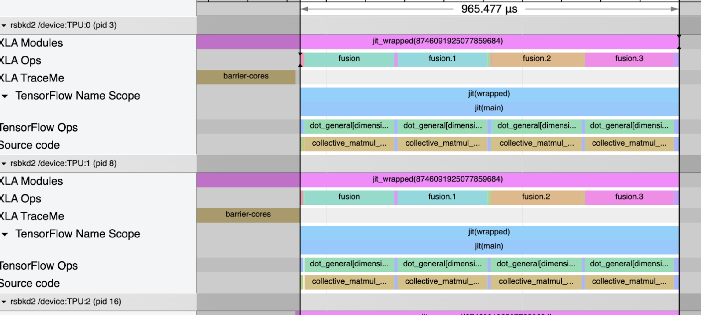
A profile shows that the all-gather is gone, and replaced with overlapped matmul with async collective permute. This profile matches very closely with the collective matmul paper result.
This collective matmul technique can be used to speed up feedforward blocks in
transformer layers. This typically consists of two matrix multiplications
followed by a ReduceScatter (to resolve partial sums from a parallelized
matrix multiplication) and preceded by an AllGather (to collect the sharded
dimensions along some axes and allow partial sum computation). Together, the
ReduceScatter from one layer and the AllGather for the next amount to an
AllReduce.
In a typical profile, the two matmuls will be followed by an AllReduce, and
they will not be overlapped. Collective matmul can be used to achieve the
overlap, but is difficult to trigger, has a minimum slice size and does not yet
cover all topologies, tensor shapes and variants of collective matmul (i.e
latency and throughput optimized variants). In a recent
paper, we found a ~40% gain in many
circumstances from manually implementing collective matmul variants in shmap
style.
But it isn’t always more complex! We expect this to be a much more natural way to think about pipelined computation, and plan to do some demos of that soon!
Another realistic example#
Here’s how shmap might look in a transformer layer pass with a 2D weight
gathered pattern (paper, Sec 3.2.3 on p. 5):
def matmul_2D_wg_manual(xnorm, q_wi, layer):
  '''Calls a custom manual implementation of matmul_reducescatter'''
  # [batch, maxlen, embed.X] @ [heads.YZ, embed.X, q_wi_per_head]
  # -> (matmul)
  # -> [batch, maxlen, heads.YZ, q_wi_per_head]{x unreduced}
  # -> (reducescatter over x into X heads, B batches)
  # -> [batch, maxlen, heads.YZX, q_wi_per_head]
  with jax.named_scope('q_wi'):
    xnorm = intermediate_dtype(xnorm)
    q_wi = matmul_reducescatter(
        'bte,hed->bthd',
        xnorm,
        params.q_wi,
        scatter_dimension=(0, 2),
        axis_name='i',
        layer=layer)
   return q_wi


import partitioning.logical_to_physical as l2phys

def pjit_transformer_layer(
    hparams: HParams, layer: int, params: weights.Layer, sin: jnp.ndarray,
    cos: jnp.ndarray, kv_caches: Sequence[attention.KVCache],
    x: jnp.ndarray) -> Tuple[jnp.ndarray, jnp.ndarray, jnp.ndarray]:
  """Forward pass through a single layer, returning output, K, V."""

  def my_layer(t, axis=0):
    """Gets the parameters corresponding to a given layer."""
    return lax.dynamic_index_in_dim(t, layer, axis=axis, keepdims=False)

  # 2D: [batch.Z, time, embed.XY]
  x = _with_sharding_constraint(
      x, ('residual_batch', 'residual_time', 'residual_embed'))
  xnorm = _layernorm(x)
  # 2D: [batch, time, embed.X]
  xnorm = _with_sharding_constraint(
      xnorm, ('post_norm_batch', 'time', 'post_norm_embed'))
  # jump into manual mode where you want to optimise
  if manual:
    q_wi = shard_map(matmul_2D_wg_manual, mesh
                in_specs=(l2phys('post_norm_batch', 'time', 'post_norm_embed'),
                          l2phys('layers', 'heads', 'embed', 'q_wi_per_head')),
                out_specs=l2phys('post_norm_batch', 'time', 'heads', 'q_wi_per_head'))(xnorm, q_wi, layer)
  else:
    q_wi = jnp.einsum('bte,hed->bthd', xnorm, my_layer(params.q_wi))
    # 2D: [batch, time, heads.YZX, None]
    q_wi = _with_sharding_constraint(q_wi,
                                   ('post_norm_batch', 'time', 'heads', 'qkv'))
  q = q_wi[:, :, :, :hparams.qkv]
  q = _rope(sin, cos, q)
  # unlike in https://arxiv.org/pdf/2002.05202.pdf, PaLM implements
  # swiGLU with full d_ff dimension, rather than 2/3 scaled
  wi0 = q_wi[:, :, :, hparams.qkv:hparams.qkv + (hparams.ff // hparams.heads)]
  wi1 = q_wi[:, :, :, hparams.qkv + (hparams.ff // hparams.heads):]
  kv = jnp.einsum('bte,ezd->btzd', xnorm, my_layer(params.kv))
  k = kv[:, :, 0, :hparams.qkv]
  v = kv[:, :, 0, hparams.qkv:]
  k = _rope(sin, cos, k)

  y_att = jnp.bfloat16(attention.attend(q, k, v, kv_caches, layer))

  y_mlp = special2.swish2(wi0) * wi1
  # 2D: [batch, time, heads.YZX, None]
  y_mlp = _with_sharding_constraint(y_mlp,
                                    ('post_norm_batch', 'time', 'heads', None))

  y_fused = jnp.concatenate([y_att, y_mlp], axis=-1)
  # do the second half of the mlp and the self-attn projection in parallel
  y_out = jnp.einsum('bthd,hde->bte', y_fused, my_layer(params.o_wo))
  # 2D: [batch.Z, time, embed.XY]
  y_out = _with_sharding_constraint(
      y_out, ('residual_batch', 'residual_time', 'residual_embed'))
  z = y_out + x
  z = _with_sharding_constraint(
      z, ('residual_batch', 'residual_time', 'residual_embed'))
  return z, k, v
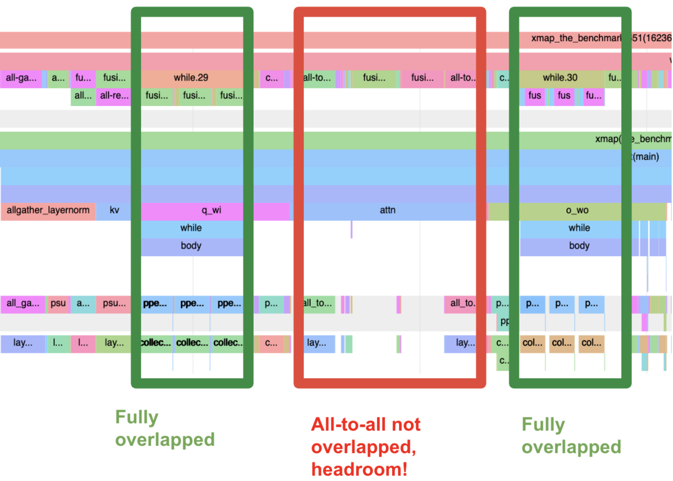
In the profile below, both the first and second matmul were replaced by manually lowered versions, where the compute (fusions) are fully overlapped with the communication (ppermute)! One fun hint that we are using a latency optimised variant is that the ppmerute pixels are jittered — because there are two overlapping ppermutes using opposite ICI axes at the same time!
All-to-all is much harder to overlap, so was left on the table.
Why don’t pmap or xmap already solve this?#
pmap was our first multi-device parallelism API. It follows the
per-device-code-and-explicit-collectives school. But it had major shortcomings
which make it unsuitable for today’s programs:
Mapping multiple axes required nested
pmaps. Not only are nestedpmaps cumbersome to write, but also they make it difficult to control (or even predict) the device placement of data and computation, and difficult to preserve data sharding (see the next two bullets). Today’s programs require multiple axes of parallelism.Controlling device placement was impossible. Especially with multiple axes of parallelism, programmers need to control how those axes are aligned with hardware resources and their communication topologies. But (nested)
pmapdoesn’t offer control over how mapped program instances are placed on hardware; there’s just an automatic device order which the user can’t control. (Gopher’s use ofaxis_index_groupsand a single un-nestedpmapwas essentially a hack to get around this by flattening multiple axes of parallelism down to one.)jit/pjitcomposability.jit-of-pmapis a performance footgun, as is nestingpmaps, as is e.g.scan-of-pmap, because sharding is not preserved when returning from an innerpmap. To preserve sharding we would need pattern matching on jaxprs to ensure we’re working with perfectly nested pmaps, or a pmap just inside ajit. Moreover,pjitwas no help here becausepmaptargets XLA replicas whilepjittargets the XLA SPMD Partitioner, and composing those two is hard.jax.Arraycompatibility (and hencepjitcompatibility). Because the sharding ofpmapoutputs can’t be expressed asShardings/OpShardings, due topmap’s stacking rather than concatenative semantics, the output of apmapcomputation can’t currently be passed to apjitcomputation without bouncing to host (or dispatching a reshaping computation).Multi-controller semantics (and hence
pjitcompatibility). Multi-controllerpmapconcatenates values across controllers, which works well but differs from single-controllerpmap’s stacking semantics. More practically, it precludes the use of non-fully-addressablejax.Arrayinputs and outputs as we use with multi-controllerpjit.Eager mode. We didn’t make
pmapeager-first, and though we eventually (after 4+ years!) added eager operation withdisable_jit(), the fact thatpmaphasjitfused into it means it has its own compilation and dispatch path (actually two dispatch paths: in Python for handlingTracers, and in C++ for performance on rawArrayinputs!), a heavy implementation burden.Reshapes needed in the caller. A typical use case with
pmapon 8 devices might look like starting with a batch axis of size 128, reshaping it to split into two axes with sizes (8, 16), and thenpmapping over the first. These reshapes are awkward and the compiler often interprets them as copies instead of view — increasing memory and time usage.
These shortcomings aren’t so bad when only doing batch data parallelism. But
when more parallelism is involved, pmap just can’t cut it!
xmap paved the way as a next-gen evolution of pmap and solved (almost) all these
issues. shmap follows in xmap’s footsteps and solves these problems in
essentially the same ways; indeed, shmap is like a specialized subset of xmap
(what some call the “hard xmap” subset), with a few tweaks.
For the initial prototype, we chose to implement shmap as a separate primitive
from xmap, because limiting the set of features it supports makes it easier to
focus on the core functionality. For example, shmap doesn’t allow unmapped
intermediates, making it easier not to worry about the interactions between
named axes and autodiff. Furthermore, not having to reason about interactions of
all pairs of features makes it easier to add capabilities beyond what’s
implemented in xmap today, such as support for eager mode.
Both shmap and xmap share significant portions of the lowering code. We
could consider merging both in the future, or even focusing solely on shmap,
depending on how the usage will evolve.